Kalman-Filters for Front-Steered Vehicles

Position tracking is a key aspect of mobile robotics. It allows the robot, to accurately follow a trajectory and put observations of the environment into context. To get an accurate position estimate, a great number of sensors and hardware configurations can be used. The methods that will be discussed in this post, however, will only focus on using an IMU (Inertial Measurement Unit) and rotary encoders on both rear wheels. The hardware setup follows the Ackermann steering geometry (as can be seen in the picture below).

Relative Position Tracking

An absolute position can be estimated by using trilateration or triangulation of detected beacons or landmarks. This method relies on prior knowledge and observability of the environment which isn't always a given. A GPS/GNSS receiver, for example, detects satellites with known locations (which act as beacons) and uses trilateration to determine its own position. Unfortunately, this method will fail when there are not enough beacons within reach of the receiver.

Relative position tracking (aka. dead reckoning) offers an alternative solution that doesn't rely on any external landmarks or beacons. Instead, the changes in speed and acceleration are used to reconstruct a trajectory and, therefore, the current position. You don't get an absolute position with respect to fixed landmarks but with the assumption that you know the starting point, you can reconstruct a position relative to that.

Using the IMU

An IMU usually combines an accelerometer and a gyroscope in one micro-electro-mechanical system (MEMS). The accelerometer measures linear accelerations along the X, Y- and Z axes, while the gyroscope measures angular velocities along those axes. A relative position can be obtained by integrating this data. It is important to note here, that the acceleration caused by the earth's gravity field, is always observed by the vehicle unless it is in free fall. This observable acceleration vector doesn't contribute to the vehicle's positional change and should, therefore, be excluded right away.

Let's assume that the vehicle is always driving on a flat plane. This means, that the gravity vector is always pointing downwards. All you need to do to get rid of it is to observe the gravity vector while the vehicle isn't moving and doesn't experience any other accelerations. Once the exact orientation and magnitude of that vector are known, it can be subtracted from all subsequent measurements. With the gravity removed, you can then simply integrate the remaining accelerations to get a position estimate.

Unfortunately, this only works under the assumption that the vehicle never changes its orientation. You have to make sure, that the accelerometer axes are always aligned with the world coordinate system. If the vehicle changes its orientation, you have to add a step to the algorithm to account for that rotation.

The discrete measurements from the gyroscope and accelerometer are numerically integrated here. This means that the result of each integration operation is the sum of all incoming measurements. The actual sensors aren't perfect however and produce error-prone and noisy data. Those errors are also summed up during the integration process as well and cause the result to drift away from its true value over time. In the picture below, you can see an example of this drift. In that setup, the double-integration method was used to estimate the position of a stationary Xsens Mtx IMU.

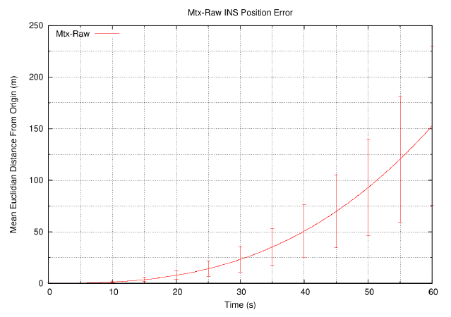
Even though the IMU wasn't moved in the experiment, the accumulated errors were causing the position to drift 50 meters after only 40 seconds. This example shows, that you should never rely on IMUs to accurately estimate a position or orientation since the time-variant drift is not just increasing fast, but exponentially.

Wheel Odometry

Another way to estimate the relative position is to utilize the rotary encoders connected to the rear wheels. This is called wheel odometry and the idea here is to observe the different travel distances of each rear wheel. If the vehicle is driving in a straight line, both rear wheels travel that same distance as well. When taking a left-hand turn, for example, the right rear wheel is traveling a longer distance than the left one. This can be used to reconstruct the trajectory of the vehicle.

To determine the current vehicle pose (pose just means position \(\color{red}{(x', y')}\) and orientation \(\color{red}{\theta'}\)), you have to add the distances \(d_{right}\) and \(d_{left}\) to the previously observed pose \(\color{red}{(x, y, \theta)}\). This is done for every new observation and results in an incremental estimation of the vehicle trajectory.

• \(d_{center} = \frac{d_{left} + d_{right}}{2}\)
• \(\varphi = \frac{d_{right} - d_{left}}{W}\)
• \(\theta' = \theta + \varphi\)
• \(x' = x + cos(\theta) \cdot d_{center}\)
• \(y' = y + sin(\theta) \cdot d_{center}\)

This numeric method only works under the assumption that \(\varphi\) has a small value and that the turning radius between the two poses doesn't change significantly. Because of that, you have to make sure that the vehicle doesn't travel too far between two calculation steps, to get reliable results. Since the rotary encoders don't measure the actual travel distance but the angular positions of each wheel (\(\delta_{left}\) and \(\delta_{right}\)), there also needs to be a translation step using the radii of the rear wheels (\(R_{left}\) and \(R_{right}\)).

• \(d_{left} = R_{left} \cdot \delta_{left}\)
• \(d_{right} = R_{right} \cdot \delta_{right}\)

Sensor Fusion

Now that we have a basic understanding of relative position tracking using either IMU or odometry data, let's try to combine both methods. The foundational paper by Borenstein and Feng (1996) describes, how these two methods can complement each other. The angular velocity of the IMU can be more accurate for short and extreme maneuvers but is noisy during slow rotations and is drifting over longer time periods. The wheel odometry, on the other hand, doesn't drift over time but becomes inaccurate when the tire rotation doesn't match the actual travel distance anymore (e.g. because of slippage or inaccurate calibration). For this reason, it might make sense to use gyroscope readings during extreme turning motions or when the vehicle traverses a bump on the ground. If you can identify these situations, you can switch between gyroscope measurements \(\varphi_{gyro}\) and odometry data \(\varphi_{odo}\) accordingly.

• \(\begin{equation} \varphi = \begin{cases} \varphi_{odo} & \text{if} \quad |\varphi_{odo} - \varphi_{gyro}| \leq \text{threshold} \\ \varphi_{gyro} & \text{else} \end{cases} \end{equation}\)

With this simple rule, we can decide which sensor is more trustworthy depending on the situation. If odometry and IMU measurements are diverging too much, it was probably caused by an extreme event which means that the IMU data is more reliable.

Kalman-Filters

Determining the reliability of sensors is also the core idea of a Kalman-Filter which takes two inputs (the control input \(u_t\) and the measurement input \(z_t\)) and assumes that the estimated state (the vehicle pose in our case) can be represented by a multivariate normal distribution. Kalman-Filters give the currently more reliable input a higher weight (aka. Kalman-Gain \(K_t\)). To get a better understanding of Kalman-Filters, I would recommend www.kalmanfilter.net or the YouTube playlist created by Michel van Biezen:

Implementation

With all the knowledge gained so far, let's try to create a Kalman-Filter that combines IMU and odometry in a way that allows each source to compensate for the other.

What you can see here, is a simple Kalman-Filter that combines IMU-data \(\color{orange}{u_t = [a_x, a_y, \omega]}\) (accelerations in XY-directions and angular velocity) and odometry data \(\color{orange}{z_t = [v_x, v_y, \varphi_{odo}]}\) (velocities in XY-directions and angular change). The previous estimation of the vehicle state \(X_{t-1}\) is used together with the IMU data to predict the current state \(\hat{X}_t\). This prediction is then updated with odometry measurements to estimate the actual current state \(X_t\). This cycle continues for every new sensor-data sample that comes in and the results can be integrated to get the desired relative position.

Instead of using the simple Gyrodometry method from before (\(|\varphi_{odo} - \varphi_{gyro}| \leq \text{threshold}\)), the covariance matrices \(Q_t\) and \(R_t\) can be used to describe how reliable the two sensors are, at every sampling point. This allows for a more elaborate model of the process and can be extended by other sensor inputs.

In reality, the approach above only offers a small improvement over Gyrodometry and doesn't make use of modern algorithms like unscented Kalman-Filters or indirect state models which would reduce errors even more. The example here just shows a simple implementation and is meant as an introduction to the topic.